Fast Download

Divide Excel Worksheet into Pages!!

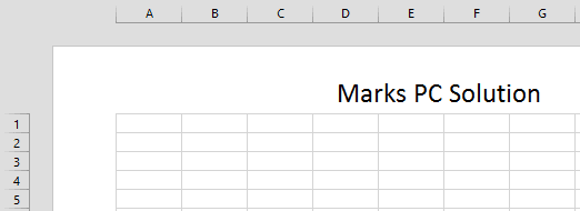
Almost all of you are familiar with the Print Layout view of Microsoft Word. Excel Page Layout view does the same job here. If you enable Page Layout view in a worksheet, you can easily understand your print area with header and footer. And it also makes your printing task easier. 

Applies to:

• Excel 2007
• Excel 2010
• Excel 2013

Advantages of Page Layout

• You can view how your printed document will look

• Check where your page begins and ends

• View headers and footers of the page

• Print the worksheet page by page

How to Enable Page Layout View

You can enable page layout view as below:

1. Open any worksheet or create a new one
2. Go to the View Tab > Workbook Views > Page Layout 

You can also use the keyboard shortcuts:

Press Alt Key > Then type WP 

If you would like to back to the Normal View then:

Press Alt Key > Then type WL 

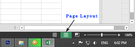
You can also enable Page Layout view from Status Bar. I think its the most handy option. Follow the image below:

The selected icon in the middle is Page Layout icon. The left one is for Normal View. And the right one is for Page Break Preview. 

Go to link download

How to Print Headings on Every Page in Excel

• MS Excel 2000/ XP

• MS Excel 2007/ 2010/ 2013

1. Open a previously saved worksheet or create a new one in MS Excel.
2. Go to the Page Setup option from Page Layout Tab (Office XP/ 2000 users should find it under Edit Menu).
3. Go to the Sheet tab from Page Setup.
4. Look at the Print titles option: Rows to repeat and Columns to repeat.
5. To repeat the headers at the top, click on the first one. Or click on the second one to repeat the columns.
6. After clicking the box, select the area of your sheet which needs to be repeated. Follow the image below.
7. Hit OK to close the Page Setup. Done! Now check by printing or look at the print preview. 

Go to link download

How to Rotate Text in Excel

Go to link download

How to Lock Rows Columns in Excel

Then I explored the topic and found the solution from Excel help and Microsoft Support Page. So, in this post, you are getting another important excel tutorial - How to Lock/ Fix/ Freeze Rows or Columns in excel while scrolling throughout the worksheet.


Lock/ Fix/ Freeze Rows or Columns

In Excel, the term is known as Freeze Panes. With this option, you can freeze a row or column that you want visible even when scrolling down or right. 

Suppose, you preparing a salary sheet that contains hundreds of rows. And you can view only 25/30 rows in a view. When you scroll down, the column headings will disappear. If you want the first row (that contains headings) visible, you have to use the Freeze Panes option. 


If youre using Office 2000/ XP/ 2003, you will get the freeze panes option under Window menu. 

1. Simply open a worksheet
2. Choose the row you wanna freeze
3. Then go to the Window menu
4. Hit on the Freeze Panes option - Done! 

If you want to unlock the row, follow the steps again, and this time you will get unfreeze option. 

For Office 2007/ 2010/ 2013

Here you will get the freeze panes option under View tab in Window section. And you can also freeze both top row and left column! 

1. Open a previously saved worksheet or create a new one.
2. Input your necessary data.
3. Go to the View Tab.
4. Find the Window section at the right and locate Freeze Panes
5. Hit on the down arrow, you will get 3 options - Freeze Panes, Freeze First Column, Freeze Tip Row.
6. Freeze Panes - Used for locking multiple rows. And the next two are used either to lock  only the first column or first row.
7. If you want to unlock the locked row or column, you have to unfreeze it by following the same steps. 

Note: Suppose you wanna freeze first 3 rows. Then you have to click on the 4th row. Now go to the Freeze Panes option in view menu and use Freeze Panes. 

Download Sample Sheet

Ive also uploaded a sample sheet which you can download from the above link. Download and open the above sample sheet. It contains the example of freezed panes. 

In the first sheet, Ive freezed a single row. In the second sheet, Ive freezed multiple rows. There you will see, first three rows are freezed. To do it, you have to put your cursor in the 4th row, then you have to choose Freeze Panes. 

Hope this will be helpful for you. In my next post, Im gonna discuss about - how to print the headings in every page. 


Reference: Freeze or Lock Rows and Columns

Go to link download

Type Multiple Lines in a Cell in Excel

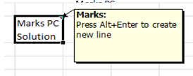
First Ive typed Marks PC, then I pressed Alt+Enter and typed Solution. But remember, first you have adjust the column size. Adjust the column size and then type your text. Once you press Alt+Enter, new lines will be creating automaticlly when the cell area ends. 


There is another shortcut for you! Just look at the image below:

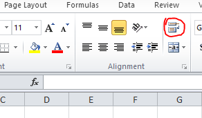
Have you noticed the market button? Its in the Alignment section, just below the Review Tab. This button is a shortcut to wrap text. Type your text and hit on this button to create multiple lines in a row/ cell. 

Go to link download

Converting Numbers into Words in Excel

• Excel 2003

• Excel 2007

• Excel 2010

• Excel 2013

• Excel 2016

Function words(fig, Optional point = "Point") As String    

Dim digit(14) As Integer    alpha = Array("", "One", "Two", "Three", "Four", "Five", "Six", "Seven", "Eight", "Nine", "Ten", "Eleven", "Twelve", "Thirteen", "Fourteen", "Fifteen", "Sixteen", "Seventeen", "Eighteen", "Nineteen", "Twenty", "Thirty", "Forty", "Fifty", "Sixty", "Seventy", "Eighty", "Ninety")    figi = Trim(StrReverse(Str(Int(Abs(fig)))))    For i = 1 To Len(figi)    digit(i) = Mid(figi, i, 1)    Next    For i = 2 To Len(figi) Step 3    If digit(i) = 1 Then    digit(i) = digit(i - 1) + 10: digit(i - 1) = 0    Else: If digit(i) > 1 Then digit(i) = digit(i) + 18    End If    Next    For i = 1 To Len(figi)    If (i Mod 3) = 0 And digit(i) > 0 Then words = "hundred " & words    If (i Mod 3) = 1 And digit(i) + digit(i + 1) + digit(i + 2) > 0 Then _    words = Choose(i / 3, "thousand ", "million ", "billion ") & words    words = Trim(alpha(digit(i)) & " " & words)    Next    If fig <> Int(fig) Then    figc = StrReverse(figi)    If figc = 0 Then figc = ""    figd = Trim(WorksheetFunction.Substitute(Str(Abs(fig)), figc & ".", ""))    words = Trim(words & " " & point)    For i = 1 To Len(figd)    If Val(Mid(figd, i, 1)) > 0 Then    words = words & " " & alpha(Mid(figd, i, 1))    Else: words = words & " Zero"    End If    Next    End If    If fig < 0 Then words = "Negative " & words    End Function

1. Open your Word Converter workbook.
2. Type a digit in a cell. i.e. type 2124 in cell C6. 
3. Put your cursor in a different cell i.e. C7.
4. Type =words(C6) in cell C7. And you will get Two thousand one hundred twenty four.

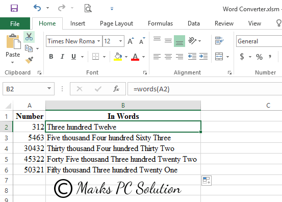
Look at the formula bar: =words(A2)

Or you can also use this method - 

1. Type your digit and put your cursor in a different cell.
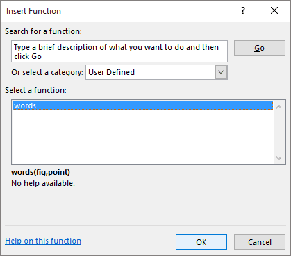
2. Go to the Formula > Insert Function > Select a Category > User Defined.
3. Now choose Words from Select a function.
4. Choose your desired cell and hit OK.

Warning Message!

When you close this document and reopen for the first time, Excel may warn you like - This document contains macro. And you should hit on the Enable Content button. If you dont hit the enable button, then word converter function may not work.

Lots of works to do ha? Seems complicated? No problem. Im sharing a sample workbook for you. Just download and do your work. :) 

Download Sample Workbook

Go to link download